https://lilianweng.github.io/posts/2017-06-21-overview

https://www.youtube.com/watch?v=F1ka6a13S9I

(The post was originated from my talk for WiMLDS x Fintech meetup hosted by Affirm.)

I believe many of you have watched or heard of the games between AlphaGo and professional Go player Lee Sedol in 2016. Lee has the highest rank of nine dan and many world championships. No doubt, he is one of the best Go players in the world, but he lost by 1-4 in this series versus AlphaGo. Before this, Go was considered to be an intractable game for computers to master, as its simple rules lay out an exponential number of variations in the board positions, many more than what in Chess. This event surely highlighted 2016 as a big year for AI. Because of AlphaGo, much attention has been attracted to the progress of AI.

Meanwhile, many companies are spending resources on pushing the edges of AI applications, that indeed have the potential to change or even revolutionize how we are gonna live. Familiar examples include self-driving cars, chatbots, home assistant devices and many others. One of the secret receipts behind the progress we have had in recent years is deep learning.

Why Does Deep Learning Work Now?

Deep learning models, in simple words, are large and deep artificial neural nets. A neural network (“NN”) can be well presented in a directed acyclic graph: the input layer takes in signal vectors; one or multiple hidden layers process the outputs of the previous layer. The initial concept of a neural network can be traced back to more than half a century ago. But why does it work now? Why do people start talking about them all of a sudden?

The reason is surprisingly simple:

• We have a lot more data.
• We have much powerful computers.

A large and deep neural network has many more layers + many more nodes in each layer, which results in exponentially many more parameters to tune. Without enough data, we cannot learn parameters efficiently. Without powerful computers, learning would be too slow and insufficient.

Here is an interesting plot presenting the relationship between the data scale and the model performance, proposed by Andrew Ng in his “Nuts and Bolts of Applying Deep Learning” talk. On a small dataset, traditional algorithms (Regression, Random Forests, SVM, GBM, etc.) or statistical learning does a great job, but once the data scale goes up to the sky, the large NN outperforms others. Partially because compared to a traditional ML model, a neural network model has many more parameters and has the capability to learn complicated nonlinear patterns. Thus we expect the model to pick the most helpful features by itself without too much expert-involved manual feature engineering.

Deep Learning Models

Next, let’s go through a few classical deep learning models.

Convolutional Neural Network

Convolutional neural networks, short for “CNN”, is a type of feed-forward artificial neural networks, in which the connectivity pattern between its neurons is inspired by the organization of the visual cortex system. The primary visual cortex (V1) does edge detection out of the raw visual input from the retina. The secondary visual cortex (V2), also called prestriate cortex, receives the edge features from V1 and extracts simple visual properties such as orientation, spatial frequency, and color. The visual area V4 handles more complicated object attributes. All the processed visual features flow into the final logic unit, inferior temporal gyrus (IT), for object recognition. The shortcut between V1 and V4 inspires a special type of CNN with connections between non-adjacent layers: Residual Net (He, et al. 2016) containing “Residual Block” which supports some input of one layer to be passed to the component two layers later.

Convolution is a mathematical term, here referring to an operation between two matrices. The convolutional layer has a fixed small matrix defined, also called kernel or filter. As the kernel is sliding, or convolving, across the matrix representation of the input image, it is computing the element-wise multiplication of the values in the kernel matrix and the original image values. Specially designed kernels can process images for common purposes like blurring, sharpening, edge detection and many others, fast and efficiently.

Convolutional and pooling (or “sub-sampling” in Fig. 4) layers act like the V1, V2 and V4 visual cortex units, responding to feature extraction. The object recognition reasoning happens in the later fully-connected layers which consume the extracted features.

Recurrent Neural Network

A sequence model is usually designed to transform an input sequence into an output sequence that lives in a different domain. Recurrent neural network, short for “RNN”, is suitable for this purpose and has shown tremendous improvement in problems like handwriting recognition, speech recognition, and machine translation (Sutskever et al. 2011, Liwicki et al. 2007).

A recurrent neural network model is born with the capability to process long sequential data and to tackle tasks with context spreading in time. The model processes one element in the sequence at one time step. After computation, the newly updated unit state is passed down to the next time step to facilitate the computation of the next element. Imagine the case when an RNN model reads all the Wikipedia articles, character by character, and then it can predict the following words given the context.

However, simple perceptron neurons that linearly combine the current input element and the last unit state may easily lose the long-term dependencies. For example, we start a sentence with “Alice is working at …” and later after a whole paragraph, we want to start the next sentence with “She” or “He” correctly. If the model forgets the character’s name “Alice”, we can never know. To resolve the issue, researchers created a special neuron with a much more complicated internal structure for memorizing long-term context, named “Long-short term memory (LSTM)” cell. It is smart enough to learn for how long it should memorize the old information, when to forget, when to make use of the new data, and how to combine the old memory with new input. This introduction is so well written that I recommend everyone with interest in LSTM to read it. It has been officially promoted in the Tensorflow documentation 😉

To demonstrate the power of RNNs, Andrej Karpathy built a character-based language model using RNN with LSTM cells. Without knowing any English vocabulary beforehand, the model could learn the relationship between characters to form words and then the relationship between words to form sentences. It could achieve a decent performance even without a huge set of training data.

RNN: Sequence-to-Sequence Model

The sequence-to-sequence model is an extended version of RNN, but its application field is distinguishable enough that I would like to list it in a separated section. Same as RNN, a sequence-to-sequence model operates on sequential data, but particularly it is commonly used to develop chatbots or personal assistants, both generating meaningful response for input questions. A sequence-to-sequence model consists of two RNNs, encoder and decoder. The encoder learns the contextual information from the input words and then hands over the knowledge to the decoder side through a “context vector” (or “thought vector”, as shown in Fig 8.). Finally, the decoder consumes the context vector and generates proper responses.

Autoencoders

Different from the previous models, autoencoders are for unsupervised learning. It is designed to learn a low-dimensional representation of a high-dimensional data set, similar to what Principal Components Analysis (PCA) does. The autoencoder model tries to learn an approximation function f(x)≈x to reproduce the input data. However, it is restricted by a bottleneck layer in the middle with a very small number of nodes. With limited capacity, the model is forced to form a very efficient encoding of the data, that is essentially the low-dimensional code we learned.

Hinton and Salakhutdinov used autoencoders to compress documents on a variety of topics. As shown in Fig 10, when both PCA and autoencoder were applied to reduce the documents onto two dimensions, autoencoder demonstrated a much better outcome. With the help of autoencoder, we can do efficient data compression to speed up the information retrieval including both documents and images.

Reinforcement (Deep) Learning

Since I started my post with AlphaGo, let us dig a bit more on why AlphaGo worked out. Reinforcement learning (“RL”) is one of the secrets behind its success. RL is a subfield of machine learning which allows machines and software agents to automatically determine the optimal behavior within a given context, with a goal to maximize the long-term performance measured by a given metric.

The Transformer Family Version 2.0

Date: January 27, 2023 | Estimated Reading Time: 45 min | Author: Lilian WengTable of Contents

Many new Transformer architecture improvements have been proposed since my last post on “The Transformer Family” about three years ago. Here I did a big refactoring and enrichment of that 2020 post — restructure the hierarchy of sections and improve many sections with more recent papers. Version 2.0 is a superset of the old version, about twice the length.

Notations

Symbol	Meaning
d	The model size / hidden state dimension / positional encoding size.
h	The number of heads in multi-head attention layer.
L	The segment length of input sequence.
N	The total number of attention layers in the model; not considering MoE.
X∈RL×d	The input sequence where each element has been mapped into an embedding vector of shape d, same as the model size.
Wk∈Rd×dk	The key weight matrix.
Wq∈Rd×dk	The query weight matrix.
Wv∈Rd×dv	The value weight matrix. Often we have dk=dv=d.
Wik,Wiq∈Rd×dk/h;Wiv∈Rd×dv/h	The weight matrices per head.
Wo∈Rdv×d	The output weight matrix.
Q=XWq∈RL×dk	The query embedding inputs.
K=XWk∈RL×dk	The key embedding inputs.
V=XWv∈RL×dv	The value embedding inputs.
qi,ki∈Rdk,vi∈Rdv	Row vectors in query, key, value matrices, Q, K and V.
Si	A collection of key positions for the i-th query qi to attend to.
A∈RL×L	The self-attention matrix between a input sequence of lenght L and itself. A=softmax(QK⊤/dk).
aij∈A	The scalar attention score between query qi and key kj.
P∈RL×d	position encoding matrix, where the i-th row pi is the positional encoding for input xi.

Transformer Basics

The Transformer (which will be referred to as “vanilla Transformer” to distinguish it from other enhanced versions; Vaswani, et al., 2017) model has an encoder-decoder architecture, as commonly used in many NMT models. Later simplified Transformer was shown to achieve great performance in language modeling tasks, like in encoder-only BERT or decoder-only GPT.

Attention and Self-Attention

Attention is a mechanism in neural network that a model can learn to make predictions by selectively attending to a given set of data. The amount of attention is quantified by learned weights and thus the output is usually formed as a weighted average.

Self-attention is a type of attention mechanism where the model makes prediction for one part of a data sample using other parts of the observation about the same sample. Conceptually, it feels quite similar to non-local means. Also note that self-attention is permutation-invariant; in other words, it is an operation on sets.

There are various forms of attention / self-attention, Transformer (Vaswani et al., 2017) relies on the scaled dot-product attention: given a query matrix Q, a key matrix K and a value matrix V, the output is a weighted sum of the value vectors, where the weight assigned to each value slot is determined by the dot-product of the query with the corresponding key:attn(Q,K,V)=softmax(QK⊤dk)V

And for a query and a key vector qi,kj∈Rd (row vectors in query and key matrices), we have a scalar score:aij=softmax(qikj⊤dk)=exp⁡(qikj⊤dk)∑r∈Siexp⁡(qikr⊤dk)

where Si is a collection of key positions for the i-th query to attend to.

See my old post for other types of attention if interested.

Multi-Head Self-Attention

The multi-head self-attention module is a key component in Transformer. Rather than only computing the attention once, the multi-head mechanism splits the inputs into smaller chunks and then computes the scaled dot-product attention over each subspace in parallel. The independent attention outputs are simply concatenated and linearly transformed into expected dimensions.MultiHeadAttn(Xq,Xk,Xv)=[head1;…;headh]Wowhere headi=Attention(XqWiq,XkWik,XvWiv)

where [.;.] is a concatenation operation. Wiq,Wik∈Rd×dk/h,Wiv∈Rd×dv/h are weight matrices to map input embeddings of size L×d into query, key and value matrices. And Wo∈Rdv×d is the output linear transformation. All the weights should be learned during training.

Encoder-Decoder Architecture

The encoder generates an attention-based representation with capability to locate a specific piece of information from a large context. It consists of a stack of 6 identity modules, each containing two submodules, a multi-head self-attention layer and a point-wise fully connected feed-forward network. By point-wise, it means that it applies the same linear transformation (with same weights) to each element in the sequence. This can also be viewed as a convolutional layer with filter size 1. Each submodule has a residual connection and layer normalization. All the submodules output data of the same dimension d.

The function of Transformer decoder is to retrieve information from the encoded representation. The architecture is quite similar to the encoder, except that the decoder contains two multi-head attention submodules instead of one in each identical repeating module. The first multi-head attention submodule is masked to prevent positions from attending to the future.

Positional Encoding

Because self-attention operation is permutation invariant, it is important to use proper positional encoding to provide order information to the model. The positional encoding P∈RL×d has the same dimension as the input embedding, so it can be added on the input directly. The vanilla Transformer considered two types of encodings:

Sinusoidal Positional Encoding

Sinusoidal positional encoding is defined as follows, given the token position i=1,…,L and the dimension δ=1,…,d:PE(i,δ)={sin⁡(i100002δ′/d)if δ=2δ′cos⁡(i100002δ′/d)if δ=2δ′+1

In this way each dimension of the positional encoding corresponds to a sinusoid of different wavelengths in different dimensions, from 2π to 10000⋅2π.

Learned Positional Encoding

Learned positional encoding assigns each element with a learned column vector which encodes its absolute position (Gehring, et al. 2017) and furthermroe this encoding can be learned differently per layer (Al-Rfou et al. 2018).

Relative Position Encoding

Shaw et al. (2018)) incorporated relative positional information into Wk and Wv. Maximum relative position is clipped to a maximum absolute value of k and this clipping operation enables the model to generalize to unseen sequence lengths. Therefore, 2k+1 unique edge labels are considered and let us denote Pk,Pv∈R2k+1 as learnable relative position representations.Aijk=Pclip(j−i,k)kAijv=Pclip(j−i,k)vwhere clip(x,k)=clip(x,−k,k)

Transformer-XL (Dai et al., 2019) proposed a type of relative positional encoding based on reparametrization of dot-product of keys and queries. To keep the positional information flow coherently across segments, Transformer-XL encodes the relative position instead, as it could be sufficient enough to know the position offset for making good predictions, i.e. i−j, between one key vector kτ,j and its query qτ,i.

If omitting the scalar 1/dk and the normalizing term in softmax but including positional encodings, we can write the attention score between query at position i and key at position j as:aij=qikj⊤=(xi+pi)Wq((xj+pj)Wk)⊤=xiWqWk⊤xj⊤+xiWqWk⊤pj⊤+piWqWk⊤xj⊤+piWqWk⊤pj⊤

Transformer-XL reparameterizes the above four terms as follows:aijrel=xiWqWEk⊤xj⊤⏟content-based addressing+xiWqWRk⊤ri−j⊤⏟content-dependent positional bias+uWEk⊤xj⊤⏟global content bias+vWRk⊤ri−j⊤⏟global positional bias

• Replace pj with relative positional encoding ri−j∈Rd;
• Replace piWq with two trainable parameters u (for content) and v (for location) in two different terms;
• Split Wk into two matrices, WEk for content information and WRk for location information.

Rotary Position Embedding

Rotary position embedding (RoPE; Su et al. 2021) encodes the absolution position with a rotation matrix and multiplies key and value matrices of every attention layer with it to inject relative positional information at every layer.

When encoding relative positional information into the inner product of the i-th key and the j-th query, we would like to formulate the function in a way that the inner product is only about the relative position i−j. Rotary Position Embedding (RoPE) makes use of the rotation operation in Euclidean space and frames the relative position embedding as simply rotating feature matrix by an angle proportional to its position index.

Given a vector z, if we want to rotate it counterclockwise by θ, we can multiply it by a rotation matrix to get Rz where the rotation matrix R is defined as:R=[cos⁡θ−sin⁡θsin⁡θcos⁡θ]

When generalizing to higher dimensional space, RoPE divide the d-dimensional space into d/2 subspaces and constructs a rotation matrix R of size d×d for token at position i:RΘ,id=[cos⁡iθ1−sin⁡iθ100…00sin⁡iθ1cos⁡iθ100…0000cos⁡iθ2−sin⁡iθ2…0000sin⁡iθ2cos⁡iθ2…00⋮⋮⋮⋮⋱⋮⋮0000…cos⁡iθd/2−sin⁡iθd/20000…sin⁡iθd/2cos⁡iθd/2]

where in the paper we have Θ=θi=10000−2(i−1)/d,i∈[1,2,…,d/2]. Note that this is essentially equivalent to sinusoidal positional encoding but formulated as a rotation matrix.

Then both key and query matrices incorporates the positional information by multiplying with this rotation matrix:qi⊤kj=(RΘ,idWqxi)⊤(RΘ,jdWkxj)=xi⊤WqRΘ,j−idWkxj where RΘ,j−id=(RΘ,id)⊤RΘ,jd

Longer Context

The length of an input sequence for transformer models at inference time is upper-bounded by the context length used for training. Naively increasing context length leads to high consumption in both time (O(L2d)) and memory (O(L2)) and may not be supported due to hardware constraints.

This section introduces several improvements in transformer architecture to better support long context at inference; E.g. using additional memory, design for better context extrapolation, or recurrency mechanism.

Context Memory

The vanilla Transformer has a fixed and limited attention span. The model can only attend to other elements in the same segments during each update step and no information can flow across separated fixed-length segments. This context segmentation causes several issues:

• The model cannot capture very long term dependencies.
• It is hard to predict the first few tokens in each segment given no or thin context.
• The evaluation is expensive. Whenever the segment is shifted to the right by one, the new segment is re-processed from scratch, although there are a lot of overlapped tokens.

Transformer-XL (Dai et al., 2019; “XL” means “extra long”) modifies the architecture to reuse hidden states between segments with an additional memory. The recurrent connection between segments is introduced into the model by continuously using the hidden states from the previous segments.

Let’s label the hidden state of the n-th layer for the (τ+1)-th segment in the model as hτ+1(n)∈RL×d. In addition to the hidden state of the last layer for the same segment hτ+1(n−1), it also depends on the hidden state of the same layer for the previous segment hτ(n). By incorporating information from the previous hidden states, the model extends the attention span much longer in the past, over multiple segments.h~τ+1(n−1)=[stop-gradient(hτ(n−1))∘hτ+1(n−1)]Qτ+1(n)=hτ+1(n−1)WqKτ+1(n)=h~τ+1(n−1)WkVτ+1(n)=h~τ+1(n−1)Wvhτ+1(n)=transformer-layer(Qτ+1(n),Kτ+1(n),Vτ+1(n))

Note that both keys and values rely on extended hidden states, while queries only consume hidden states at the current step. The concatenation operation [.∘.] is along the sequence length dimension. And Transformer-XL needs to use relative positional encoding because previous and current segments would be assigned with the same encoding if we encode absolute positions, which is undesired.

Compressive Transformer (Rae et al. 2019) extends Transformer-XL by compressing past memories to support longer sequences. It explicitly adds memory slots of size mm per layer for storing past activations of this layer to preserve long context. When some past activations become old enough, they are compressed and saved in an additional compressed memory of size mcm per layer.

Both memory and compressed memory are FIFO queues. Given the model context length L, the compression function of compression rate c is defined as fc:RL×d→R[Lc]×d, mapping L oldest activations to [Lc] compressed memory elements. There are several choices of compression functions:

1. Max/mean pooling of kernel and stride size c;
2. 1D convolution with kernel and stride size c (need to learn additional parameters);
3. Dilated convolution (need to learn additional parameters). In their experiments, convolution compression works out the best on EnWik8 dataset;
4. Most used memories.

Compressive transformer has two additional training losses:

1. Auto-encoding loss (lossless compression objective) measures how well we can reconstruct the original memories from compressed memoriesLac=‖old_mem(i)−g(new_cm(i))‖2where g:R[Lc]×d→RL×d reverses the compression function f.
2. Attention-reconstruction loss (lossy objective) reconstructs content-based attention over memory vs compressed memory and minimize the difference:Lar=‖attn(h(i),old_mem(i))−attn(h(i),new_cm(i))‖2

Transformer-XL with a memory of size m has a maximum temporal range of m×N, where N is the number of layers in the model, and attention cost O(L2+Lm). In comparison, compressed transformer has a temporal range of (mm+c⋅mcm)×N and attention cost O(L2+L(mm+mcm)). A larger compression rate c gives better tradeoff between temporal range length and attention cost.

Attention weights, from oldest to newest, are stored in three locations: compressed memory → memory → causally masked sequence. In the experiments, they observed an increase in attention weights from oldest activations stored in the regular memory, to activations stored in the compressed memory, implying that the network is learning to preserve salient information.

Non-Differentiable External Memory

kNN-LM (Khandelwal et al. 2020) enhances a pretrained LM with a separate kNN model by linearly interpolating the next token probabilities predicted by both models. The kNN model is built upon an external key-value store which can store any large pre-training dataset or OOD new dataset. This datastore is preprocessed to save a large number of pairs, (LM embedding representation of context, next token) and the nearest neighbor retrieval happens in the LM embedding space. Because the datastore can be gigantic, we need to rely on libraries for fast dense vector search such as FAISS or ScaNN. The indexing process only happens once and parallelism is easy to implement at inference time.

At inference time, the next token probability is a weighted sum of two predictions:𝟙p(y|x)=λpkNN(y|x)+(1−λ)pLM(y|x)pkNN(y|x)∝∑(ki,wi)∈N1[y=wi]exp⁡(−d(ki,f(x)))

where N contains a set of nearest neighbor data points retrieved by kNN; d(.,.) is a distance function such as L2 distance.

According to the experiments, larger datastore size or larger k is correlated with better perplexity. The weighting scalar λ should be tuned, but in general it is expected to be larger for out-of-domain data compared to in-domain data and larger datastore can afford a larger λ.

SPALM (Adaptive semiparametric language models; Yogatama et al. 2021) incorporates both (1) Transformer-XL style memory for hidden states from external context as short-term memory and (2) kNN-LM style key-value store as long memory.

SPALM runs kNN search to fetch k tokens with most relevant context. For each token we can get the same embedding representation provided by a pretrained LM, denoted as {yi}i=1k. The gating mechanism first aggregates the retrieved token embeddings with a simple attention layer using htR (the hidden state for token xt at layer R) as a query and then learns a gating parameter gt to balance between local information htR and long-term information mt.mt=∑i=1kexp⁡(yi⊤htR)∑j=1kexp⁡(yj⊤htR)⋅yigt=σ(wg⊤htR)zt=(1−gt)⊙mt+gt⊙htRp(xt+1∣x≤t)=softmax(zt;W)

where wg is a parameter vector to learn; σ(.) is sigmoid; W is the word embedding matrix shared between both input and output tokens. Different from kNN-LM, they didn’t find the nearest neighbor distance to be helpful in the aggregation of retrieved tokens.

During training, the key representations in the long-term memory stay constant, produced by a pretrained LM, but the value encoder, aka the word embedding matrix, gets updated.

Memorizing Transformer (Wu et al. 2022) adds a kNN-augmented attention layer near the top stack of a decoder-only Transformer. This special layer maintains a Transformer-XL style FIFO cache of past key-value pairs.

The same QKV values are used for both local attention and kNN mechanisms. The kNN lookup returns top-k (key, value) pairs for each query in the input sequence and then they are processed through the self-attention stack to compute a weighted average of retrieved values. Two types of attention are combined with a learnable per-head gating parameter. To prevent large distributional shifts in value magnitude, both keys and values in the cache are normalized.

What they found during experiments with Memorizing Transformer:

• It is observed in some experiments that training models with a small memory and then finetuned with a larger memory works better than training with a large memory from scratch.
• The smaller Memorizing Transformer with just 8k tokens in memory can match the perplexity of a larger vanilla Transformer with 5X more trainable parameters.
• Increasing the size of external memory provided consistent gains up to a size of 262K.
• A non-memory transformer can be finetuned to use memory.

Distance-Enhanced Attention Scores

Distance Aware Transformer(DA-Transformer; Wu, et al. 2021) and Attention with Linear Biases (ALiBi; Press et al. 2022) are motivated by similar ideas — in order to encourage the model to extrapolate over longer context than what the model is trained on, we can explicitly attach the positional information to every pair of attention score based on the distance between key and query tokens.

Note that the default positional encoding in vanilla Transformer only adds positional information to the input sequence, while later improved encoding mechanisms alter attention scores of every layer, such as rotary position embedding, and they take on form very similar to distance enhanced attention scores.

DA-Transformer (Wu, et al. 2021) multiplies attention scores at each layer by a learnable bias that is formulated as a function of the distance between key and query. Different attention heads use different parameters to distinguish diverse preferences to short-term vs long-term context. Given two positions, i,j, DA-Transformer uses the following weighting function to alter the self-attention score:R(i)=αiRwhere Rij=|i−j|f(R(i);βi)=1+exp⁡(βi)1+exp⁡(βi−R(i))attn(Q(i),K(i),V(i))=row-softmax(ReLU(Q(i)K(i)⊤)f(R(i))d)V(i)

where αi is a learnable parameters to weight relative distance differently per head where the head is indexed by superscript (i); βi is a learnable parameter to control the upper bound and ascending slope wrt the distance for the i-th attention head. The weighting function f(.) is designed in a way that: (1) f(0)=1; (2) f(R(i))=0 when R(i)→−∞; (3) f(R(i)) is bounded when R(i)→+∞; (4) the scale is tunable; (5) and the function is monotonic. The extra time complexity brought by f(R(i)) is O(L2) and it is small relative to the self attention time complexity O(L2d). The extra memory consumption is minimal, ~O(2h).

Instead of multipliers, ALiBi (Press et al. 2022) adds a constant bias term on query-key attention scores, proportional to pairwise distances. The bias introduces a strong recency preference and penalizes keys that are too far away. The penalties are increased at different rates within different heads.softmax(qiK⊤+αi⋅[0,−1,−2,…,−(i−1)])where αi is a head-specific weighting scalar. Different from DA-transformer, αi is not learned but fixed as a geometric sequence; for example, for 8 heads, αi=12,122,…,128. The overall idea is very much similar to what relative positional encoding aims to solve.

With ALiBi, Press et al. (2022) trained a 1.3B model on context length 1024 during training and extrapolated to 2046 at inference time.

Make it Recurrent

Universal Transformer (Dehghani, et al. 2019) combines self-attention in Transformer with the recurrent mechanism in RNN, aiming to benefit from both a long-term global receptive field of Transformer and learned inductive biases of RNN. Rather than going through a fixed number of layers, Universal Transformer dynamically adjusts the number of steps using adaptive computation time. If we fix the number of steps, an Universal Transformer is equivalent to a multi-layer Transformer with shared parameters across layers.

On a high level, the universal transformer can be viewed as a recurrent function for learning the hidden state representation per token. The recurrent function evolves in parallel across token positions and the information between positions is shared through self-attention.

Given an input sequence of length L, Universal Transformer iteratively updates the representation ht∈RL×d at step t for an adjustable number of steps. At step 0, h0 is initialized to be same as the input embedding matrix. All the positions are processed in parallel in the multi-head self-attention mechanism and then go through a recurrent transition function.At=LayerNorm(ht−1+MultiHeadAttention(ht−1+Pt)ht=LayerNorm(At−1+Transition(At))

where Transition(.) is either a separable convolution or a fully-connected neural network that consists of two position-wise (i.e. applied to each row of At individually) affine transformation + one ReLU.

The positional encoding Pt uses sinusoidal position signal but with an additional time dimension:PE(i,t,δ)={sin⁡(i100002δ′/d)⊕sin⁡(t100002δ′/d)if δ=2δ′cos⁡(i100002δ′/d)⊕cos⁡(t100002δ′/d)if δ=2δ′+1

In the adaptive version of Universal Transformer, the number of recurrent steps T is dynamically determined by ACT. Each position is equipped with a dynamic ACT halting mechanism. Once a per-token recurrent block halts, it stops taking more recurrent updates but simply copies the current value to the next step until all the blocks halt or until the model reaches a maximum step limit.

Adaptive Modeling

Adaptive modeling refers to a mechanism that can adjust the amount of computation according to different inputs. For example, some tokens may only need local information and thus demand a shorter attention span; Or some tokens are relatively easier to predict and do not need to be processed through the entire attention stack.

Adaptive Attention Span

One key advantage of Transformer is the capability of capturing long-term dependencies. Depending on the context, the model may prefer to attend further sometime than others; or one attention head may had different attention pattern from the other. If the attention span could adapt its length flexibly and only attend further back when needed, it would help reduce both computation and memory cost to support longer maximum context size in the model.

This is the motivation for Adaptive Attention Span. Sukhbaatar et al (2019) proposed a self-attention mechanism that seeks an optimal attention span. They hypothesized that different attention heads might assign scores differently within the same context window (See Fig. 14) and thus the optimal span would be trained separately per head.

Given the i-th token, we need to compute the attention weights between this token and other keys within its attention span of size s:eij=qikj⊤aij=softmax(eij)=exp⁡(eij)∑r=i−si−1exp⁡(eir)yi=∑r=i−si−1airvr=∑r=i−si−1airxrWv

A soft mask function mz is added to control for an effective adjustable attention span, which maps the distance between query and key into a [0, 1] value. mz is parameterized by z∈[0,s] and z is to be learned:mz(x)=clip(1R(R+z−x),0,1)

where R is a hyper-parameter which defines the softness of mz.

The soft mask function is applied to the softmax elements in the attention weights:aij=mz(i−j)exp⁡(sij)∑r=i−si−1mz(i−r)exp⁡(sir)

In the above equation, z is differentiable so it is trained jointly with other parts of the model. Parameters z(i),i=1,…,h are learned separately per head. Moreover, the loss function has an extra L1 penalty on ∑i=1hz(i).

Using Adaptive Computation Time, the approach can be further enhanced to have flexible attention span length, adaptive to the current input dynamically. The span parameter zt of an attention head at time t is a sigmoidal function, zt=Sσ(v⋅xt+b), where the vector v and the bias scalar b are learned jointly with other parameters.

In the experiments of Transformer with adaptive attention span, Sukhbaatar, et al. (2019) found a general tendency that lower layers do not require very long attention spans, while a few attention heads in higher layers may use exceptionally long spans. Adaptive attention span also helps greatly reduce the number of FLOPS, especially in a big model with many attention layers and a large context length.

Depth-Adaptive Transformer

At inference time, it is natural to assume that some tokens are easier to predict and thus do not require as much computation as others. Therefore we may only process its prediction through a limited number of layers to achieve a good balance between speed and performance.

Both Depth-Adaptive Transformer (Elabyad et al. 2020) and Confident Adaptive Language Model (CALM; Schuster et al. 2022) are motivated by this idea and learn to predict optimal numbers of layers needed for different input tokens.

Depth-adaptive transformer (Elabyad et al. 2020) attaches an output classifier to every layer to produce exit predictions based on activations of that layer. The classifier weight matrices can be different per layer or shared across layers. During training, the model sample different sequences of exits such that the model is optimized with hidden states of different layers. The learning objective incorporates likelihood probabilities predicted at different layers, n=1,…,N:LLtn=log⁡p(yt|ht−1n)LLn=∑t=1|y|LLtn

Adaptive depth classifiers outputs a parametric distribution qt. It is trained with cross entropy loss against an oracle distribution qt∗. The paper explored three confiurations for how to learn such a classifier qt.

1. Sequence-specific depth classifier: All tokens of the same sequence share the same exit block. It depends on the average of the encoder representation of the sequence. Given an input sequence x of length L, the classifier takes x¯=1L∑t=1Lxt as input and outputs a multinomial distribution of N dimensions, corresponding to N layers.q(n|x)=softmax(Wnx¯+bn)∈RNqlik∗(x,y)=δ(arg⁡maxnLLn−λn)or qcorr∗(x,y)=δ(arg⁡maxnCn−λn) where Cn=|{t|yt=arg⁡maxyp(y|ht−1n)}|where δ is dirac delta (unit impulse) function and −λn is a regularization term to encourage lower layer exits. The ground truth q∗ can be prepared in two way, based on maximum likelihood qlik∗ or correctness qcorr∗.
   
2. Token-specific depth classifier (multinomial): Each token is decoded with different exit block, predicted conditioned on the first decoder hidden state ht1:qt(n|x,y<t)=softmax(Wnht1+bn)
3. Token-specific depth classifier (geometric-like): A binary exit prediction distribution is made per layer per token, Xtn. The RBF kernel κ(t,t′)=exp⁡(|t−t′|2σ) is used to smooth the predictions to incorporate the impact of current decision on future time steps.𝟙Xtn=sigmoid(wn⊤htn+bn)∀n∈[1,…,N−1]qt(n|x,y<t)={Xtn∏n′<n(1−Xtn′)if n<N∏n′<N(1−Xtn′)otherwiseqlik∗(x,y)=δ(arg⁡maxnLL~tn−λn) where LL~tn=∑t′=1|y|κ(t,t′)LLt′nor qcor∗(x,y)=δ(arg⁡maxnC~tn−λn) where Ctn=1[yt=arg⁡maxyp(y|ht−1n)],C~tn=∑t′=1|y|κ(t,t′)Ct′n

At inference time, the confidence threshold for making an exit decision needs to be calibrated. Depth-adaptive transformer finds such a threshold on a validation set via grid search. CALM (Schuster et al. 2022) applied the Learn then Test (LTT) framework (Angelopoulos et al. 2021) to identify a subset of valid thresholds and chose the minimum value as the threshold for inference. Except for training per-layer exit classifier, CALM also explored other methods for adaptive depth prediction, including the softmax responses (i.e. difference between top two softmax outputs) and hidden state saturation (i.e. cos⁡(htn,htn+1)) as confidence scores for exit decisions. They found softmax responses result in best inference speedup.

Efficient Attention

The computation and memory cost of the vanilla Transformer grows quadratically with sequence length and hence it is hard to be applied on very long sequences. Many efficiency improvements for Transformer architecture have something to do with the self-attention module – making it cheaper, smaller or faster to run. See the survey paper on Efficient Transformers (Tay et al. 2020).

Sparse Attention Patterns

Fixed Local Context

A simple alternation to make self-attention less expensive is to restrict the attention span of each token to local context only, so that self-attention grows linearly with the sequence length.

The idea was introduced by Image Transformer (Parmer, et al 2018), which formulates image generation as sequence modeling using an encoder-decoder transformer architecture:

• The encoder generates a contextualized, per-pixel-channel representation of the source image;
• Then the decoder autoregressively generates an output image, one channel per pixel at each time step.

Let’s label the representation of the current pixel to be generated as the query q. Other positions whose representations will be used for computing q are key vector k1,k2,… and they together form a memory matrix M. The scope of M defines the context window for pixel query q.

Image Transformer introduced two types of localized M, as illustrated below.

1. 1D Local Attention: The input image is flattened in the raster scanning order, that is, from left to right and top to bottom. The linearized image is then partitioned into non-overlapping query blocks. The context window consists of pixels in the same query block as q and a fixed number of additional pixels generated before this query block.
   
2. 2D Local Attention: The image is partitioned into multiple non-overlapping rectangular query blocks. The query pixel can attend to all others in the same memory blocks. To make sure the pixel at the top-left corner can also have a valid context window, the memory block is extended to the top, left and right by a fixed amount, respectively.

Strided Context

Sparse Transformer (Child et al., 2019) introduced factorized self-attention, through sparse matrix factorization, making it possible to train dense attention networks with hundreds of layers on sequence length up to 16,384, which would be infeasible on modern hardware otherwise.

Given a set of attention connectivity pattern S={S1,…,Sn}, where each Si records a set of key positions that the i-th query vector attends to.Attend(X,S)=(a(xi,Si))i∈{1,…,L} where a(xi,Si)=softmax((xiWq)(xjWk)j∈Si⊤dk)(xjWv)j∈Si

Note that although the size of Si is not fixed, a(xi,Si) is always of size dv and thus Attend(X,S)∈RL×dv.

In auto-regressive models, one attention span is defined as Si={j:j≤i} as it allows each token to attend to all the positions in the past.

In factorized self-attention, the set Si is decomposed into a tree of dependencies, such that for every pair of (i,j) where j≤i, there is a path connecting i back to j and i can attend to j either directly or indirectly.

Precisely, the set Si is divided into p non-overlapping subsets, where the m-th subset is denoted as Ai(m)⊂Si,m=1,…,p. Therefore the path between the output position i and any j has a maximum length p+1. For example, if (j,a,b,c,…,i) is a path of indices between i and j, we would have j∈Aa(1),a∈Ab(2),b∈Ac(3),…, so on and so forth.

Sparse Factorized Attention

Sparse Transformer proposed two types of fractorized attention. It is easier to understand the concepts as illustrated in Fig. 10 with 2D image inputs as examples.

1. Strided attention with stride ℓ∼n. This works well with image data as the structure is aligned with strides. In the image case, each pixel would attend to all the previous ℓ pixels in the raster scanning order (naturally cover the entire width of the image) and then those pixels attend to others in the same column (defined by another attention connectivity subset).Ai(1)={t,t+1,…,i}, where t=max(0,i−ℓ)Ai(2)={j:(i−j)modℓ=0}
2. Fixed attention. A small set of tokens summarize previous locations and propagate that information to all future locations.Ai(1)={j:⌊jℓ⌋=⌊iℓ⌋}Ai(2)={j:jmodℓ∈{ℓ−c,…,ℓ−1}}where c is a hyperparameter. If c=1, it restricts the representation whereas many depend on a few positions. The paper chose c∈{8,16,32} for ℓ∈{128,256}.

Use Factorized Self-Attention in Transformer

There are three ways to use sparse factorized attention patterns in Transformer architecture:

1. One attention type per residual block and then interleave them,
   attn(X)=Attend(X,A(nmodp))Wo, where n is the index of the current residual block.
2. Set up a single head which attends to locations that all the factorized heads attend to,
   attn(X)=Attend(X,∪m=1pA(m))Wo.
3. Use a multi-head attention mechanism, but different from vanilla Transformer, each head might adopt a pattern presented above, 1 or 2. → This option often performs the best.

Sparse Transformer also proposed a set of changes so as to train the Transformer up to hundreds of layers, including gradient checkpointing, recomputing attention & FF layers during the backward pass, mixed precision training, efficient block-sparse implementation, etc. Please check the paper for more details or my previous post on techniques for scaling up model training.

Blockwise Attention (Qiu et al. 2019) introduces a sparse block matrix to only allow each token to attend to a small set of other tokens. Each attention matrix of size L×L is partitioned into n×n smaller blocks of size Ln×Ln and a sparse block matrix M∈{0,1}L×L is defined by a permutation π of 1,…,n, which records the column index per row in the block matrix.attn(Q,K,V,M)=softmax(QK⊤d⊙M)V(A⊙M)ij={Aijif Mij=1−∞if Mij=0where Mij={1if π(⌊(i−1)nL+1⌋)=⌊(j−1)nL+1⌋0otherwise

The actual implementation of Blockwise Attention only stores QKV as block matrices, each of size n×n:Blockwise-attn(Q,K,V,M)=[softmax(q^1k^π(1)⊤d)v^π(1)⋮softmax(q^nk^π(n)⊤d⊙)v^π(n)]

where q^i, k^i and v^i are the i-the row in the QKV block matrix respectively. Each qikπ(i)⊤,∀i=1,…,n is of size Nn×Nn and therefore Blockwise Attention is able to reduce the memory complexity of attention matrix from O(L2) to O(Ln×Ln×n)=O(L2/n).

Combination of Local and Global Context

ETC (Extended Transformer Construction; Ainslie et al. 2019), Longformer (Beltagy et al. 2020) and Big Bird (Zaheer et al. 2020) models combine both local and global context when building an attention matrix. All these models can be initialized from existing pretrained models.

Global-Local Attention of ETC (Ainslie et al. 2019) takes two inputs, (1) the long input xl of size nl which is the regular input sequence and (2) the global input xg of size ng which contains a smaller number of auxiliary tokens, ng≪nl. Attention is thus split into four components based on directional attention across these two inputs: g2g, g2l, l2g and l2l. Because the l2l attention piece can be very large, it is restricted to a fixed size attention span of radius w (i.e. local attention span) and the l2l matrix can be reshaped to nl×(2w+1).

ETC utilizes four binary matrices to handle structured inputs, Mg2g, Mg2l, Ml2g and Ml2l. For example, each element zig∈Rd in the attention output zg=(z1g,…,zngg) for g2g attention piece is formatted as:aijg2g=1dxigWQ(xjgWK+PijK)⊤−(1−Mijg2g)CAijg2g=exp⁡(aijg2g)∑k=1ngexp⁡(aikg2g)zig=∑j=1ngAijg2gxjgWV

where PijK is a learnable vector for relative position encoding and C is a very large constant (C=10000 in the paper) to offset any attention weights when mask is off.

One more update in ETC is to incorporate a CPC (contrastive predictive coding) task using NCE loss into the pretraining stage, besides the MLM task: The representation of one sentence should be similar to the representation of context around it when this sentence is masked.

The global input xg for ETC is constructed as follows: Assuming there are some segments within the long inputs (e.g. by sentence), each segment is attached with one auxiliary token to learn global inputs. Relative position encoding is used to mark the global segment tokens with the token position. Hard masking in one direction (i.e., tokens before vs after are labeled differently) is found to bring performance gains in some datasets.

Attention pattern in Longformer contains three components:

1. Local attention: Similar to ETC, local attention is controlled by a sliding window of fixed size w;
2. Global attention of preselected tokens: Longformer has a few pre-selected tokens (e.g. [CLS] token) assigned with global attention span, that is, attending to all other tokens in the input sequence.
3. Dilated attention: Dilated sliding window of fixed size r and gaps of dilation size d, similar to Sparse Transformer;

Big Bird is quite similar to Longformer, equipped with both local attention and a few preselected tokens with global attention span, but Big Bird replaces dilated attention with a new mechanism where all tokens attend to a set of random tokens. The design is motivated by the fact that attention pattern can be viewed as a directed graph and a random graph has the property that information is able to rapidly flow between any pair of nodes.

Longformer uses smaller window size at lower layers and larger window sizes at higher layers. Ablation studies showed that this setup works better than reversed or fixed size config. Lower layers do not have dilated sliding windows to better learn to use immediate local context. Longformer also has a staged training procedure where initially the model is trained with small window size to learn from local context and then subsequent stages of training have window sizes increased and learning rate decreased.

Content-based Attention

The improvements proposed by Reformer (Kitaev, et al. 2020) aim to solve the following pain points in vanilla Transformer:

• Quadratic time and memory complexity within self-attention module.
• Memory in a model with N layers is N-times larger than in a single-layer model because we need to store activations for back-propagation.
• The intermediate FF layers are often quite large.

Reformer proposed two main changes:

1. Replace the dot-product attention with locality-sensitive hashing (LSH) attention, reducing the complexity from O(L2) to O(Llog⁡L).
2. Replace the standard residual blocks with reversible residual layers, which allows storing activations only once during training instead of N times (i.e. proportional to the number of layers).

Locality-Sensitive Hashing Attention

In QK⊤ part of the attention formula, we are only interested in the largest elements as only large elements contribute a lot after softmax. For each query qi∈Q, we are looking for row vectors in K closest to qi. In order to find nearest neighbors quickly in high-dimensional space, Reformer incorporates Locality-Sensitive Hashing (LSH) into its attention mechanism.

A hashing scheme x↦h(x) is locality-sensitive if it preserves the distancing information between data points, such that close vectors obtain similar hashes while distant vectors have very different ones. The Reformer adopts a hashing scheme as such, given a fixed random matrix R∈Rd×b/2 (where b is a hyperparam), the hash function is h(x)=arg⁡max([xR;−xR]).

In LSH attention, a query can only attend to positions in the same hashing bucket, Si={j:h(qi)=h(kj)}. It is carried out in the following process, as illustrated in Fig. 20:

• (a) The attention matrix for full attention is often sparse.
• (b) Using LSH, we can sort the keys and queries to be aligned according to their hash buckets.
• (c) Set Q=K (precisely kj=qj/|qj|), so that there are equal numbers of keys and queries in one bucket, easier for batching. Interestingly, this “shared-QK” config does not affect the performance of the Transformer.
• (d) Apply batching where chunks of m consecutive queries are grouped together.

Reversible Residual Network

Another improvement by Reformer is to use reversible residual layers (Gomez et al. 2017). The motivation for reversible residual network is to design the architecture in a way that activations at any given layer can be recovered from the activations at the following layer, using only the model parameters. Hence, we can save memory by recomputing the activation during backprop rather than storing all the activations.

Given a layer x↦y, the normal residual layer does y=x+F(x), but the reversible layer splits both input and output into pairs (x1,x2)↦(y1,y2) and then executes the following:y1=x1+F(x2),y2=x2+G(y1)

and reversing is easy:x2=y2−G(y1),x1=y1−F(x2)

Reformer applies the same idea to Transformer by combination attention (F) and feed-forward layers (G) within a reversible net block:Y1=X1+Attention(X2),Y2=X2+FeedForward(Y1)

The memory can be further reduced by chunking the feed-forward computation:Y2=[Y2(1);…;Y2(c)]=[X2(1)+FeedForward(Y1(1));…;X2(c)+FeedForward(Y1(c))]

The resulting reversible Transformer does not need to store activation in every layer.

Routing Transformer (Roy et al. 2021) is also built on content-based clustering of keys and queries. Instead of using a static hashing function like LSH, it utilizes online k-means clustering and combines it with local, temporal sparse attention to reduce the attention complexity from O(L2) to O(L1.5).

Within routing attention, both keys and queries are clustered with k-means clustering method and the same set of centroids μ=(μ1,…,μk)∈Rk×d. Queries are routed to keys that get assigned to the same centroid. The total complexity is O(Lkd+L2d/k), where O(Lkd) is for running clustering assignments and O(L2d/k) is for attention computation. The cluster centroids are updated by EMA (exponential moving average) using all associated keys and queries.

In the experiments for Routing Transformer, some best config only has routing attention enabled in the last two layers of the model and half of the attention heads, while the other half utilizing local attention. They also observed that local attention is a pretty strong baseline and larger attention window always leads to better results.

Low-Rank Attention

Linformer (Wang et al. 2020) approximates the full attention matrix with a low rank matrix, reducing the time & space complexity to be linear. Instead of using expensive SVD to identify low rank decomposition, Linformer adds two linear projections Ei,Fi∈RL×k for key and value matrices, respectively, reducing their dimensions from L×d to k×d. As long as k≪L, the attention memory can be greatly reduced.head―i=attn(XqWiq,EiXkWik,FiXvWiv)=softmax(XqWiq(EiXkWik)⊤d)⏟low rank attention matrix A¯∈Rk×dFiXvWiv

Additional techniques can be applied to further improve efficiency of Linformer:

• Parameter sharing between projection layers, such as head-wise, key-value and layer-wise (across all layers) sharing.
• Use different k at different layers, as heads in higher layers tend to have a more skewed distribution (lower rank) and thus we can use smaller k at higher layers.
• Use different types of projections; e.g. mean/max pooling, convolution layer with kernel and stride L/k.

Random Feature Attention (RFA; Peng et al. 2021) relies on random feature methods (Rahimi & Recht, 2007) to approximate softmax operation in self-attention with low rank feature maps in order to achieve linear time and space complexity. Performers (Choromanski et al. 2021) also adopts random feature attention with improvements on the kernel construction to further reduce the kernel approximation error.

The main theorem behind RFA is from Rahimi & Recht, 2007:

Let ϕ:Rd→R2D be a nonlinear transformation:ϕ(x)=1D[sin⁡(w1⊤x),…,sin⁡(wD⊤x),cos⁡(w1⊤x),…,cos⁡(wD⊤x)]⊤

When d

-dimensional random vectors wi

 are i.i.d. from N(0,σ2Id)

,Ewi[ϕ(x)⋅ϕ(y)]=exp⁡(−‖x−y‖22σ2)

An unbiased estimation of exp⁡(x⋅y) is:exp⁡(x⋅y/σ2)=exp⁡(12σ2(‖x‖2+‖y‖2−‖x−y‖2)=exp⁡(‖x‖22σ2)exp⁡(‖y‖22σ2)(−‖x−y‖22σ2)≈exp⁡(‖x‖22σ2)exp⁡(‖y‖22σ2)ϕ(x)⋅ϕ(y)=exp⁡(1σ2)ϕ(x)⋅ϕ(y); unit vectors

Then we can write the attention function as follows, where ⊗ is outer product operation and σ2 is the temperature:attn(qt,{ki},{vi})=∑iexp⁡(qt⋅ki/σ2)∑jexp⁡(qt⋅kj/σ2)vi⊤≈∑iϕ(qt)ϕ(ki)vi⊤∑jϕ(qt)ϕ(kj)=ϕ(qt)⊤∑iϕ(ki)⊗viϕ(qt)⊤∑jϕ(kj)=RFA(qt,{ki},{vi})

Causal Attention RFA has token at time step t only attend to earlier keys and values {ki}i≤t,{vi}i≤t. Let us use a tuple of variables, (St∈R2D×d,z∈R2D), to track the hidden state history at time step t, similar to RNNs:causal-RFA(qt,{ki}i≤t,{vi}i≤t)=ϕ(qt)⊤Stϕ(qt)⋅ztwhere St=St−1+ϕ(kt)⊗vt,zt=zt−1+ϕ(kt)

where 2D is the size of ϕ(.) and D should be no less than the model size d for reasonable approximation.

RFA leads to significant speedup in autoregressive decoding and the memory complexity mainly depends on the choice of D when constructing the kernel ϕ(.).

Performer modifies the random feature attention with positive random feature maps to reduce the estimation error. It also keeps the randomly sampled w1,…,wD to be orthogonal to further reduce the variance of the estimator.

Transformers for Reinforcement Learning

The self-attention mechanism avoids compressing the whole past into a fixed-size hidden state and does not suffer from vanishing or exploding gradients as much as RNNs. Reinforcement Learning tasks can for sure benefit from these traits. However, it is quite difficult to train Transformer even in supervised learning, let alone in the RL context. It could be quite challenging to stabilize and train a LSTM agent by itself, after all.

The Gated Transformer-XL (GTrXL; Parisotto, et al. 2019) is one attempt to use Transformer for RL. GTrXL succeeded in stabilizing training with two changes on top of Transformer-XL:

1. The layer normalization is only applied on the input stream in a residual module, but NOT on the shortcut stream. A key benefit to this reordering is to allow the original input to flow from the first to last layer.
2. The residual connection is replaced with a GRU-style (Gated Recurrent Unit; Chung et al., 2014) gating mechanism.

r=σ(Wr(l)y+Ur(l)x)z=σ(Wz(l)y+Uz(l)x−bg(l))h^=tanh⁡(Wg(l)y+Ug(l)(r⊙x))g(l)(x,y)=(1−z)⊙x+z⊙h^

The gating function parameters are explicitly initialized to be close to an identity map – this is why there is a bg term. A bg>0 greatly helps with the learning speedup.

Decision Transformer (DT; Chen et al 2021) formulates Reinforcement Learning problems as a process of conditional sequence modeling, outputting the optimal actions conditioned on the desired return, past states and actions. It therefore becomes straightforward to use Transformer architecture. Decision Transformer is for off-policy RL, where the model only has access to a fixed collection of trajectories collected by other policies.

To encourage the model to learn how to act in order to achieve a desired return, it feeds the model with desired future return R^=∑t′=tTrt′ instead of the current reward. The trajectory consists of a list of triplets, (return-to-go R^t,states_t,actiona_t$), and it is used as an input sequence for Transformer:τ=(R^1,s1,a1,R^2,s2,a2,…,R^T,sT,aT)

Three linear layers are added and trained for return-to-go, state and action respectively to extract token embeddings. The prediction head learns to predict at corresponding to the input token st. The training uses cross-entropy loss for discrete actions or MSE for continuous actions. Predicting the states or return-to-go was not found to help improve the performance in their experiments.

The experiments compared DT with several model-free RL algorithm baselines and showed that:

• DT is more efficient than behavior cloning in low data regime;
• DT can model the distribution of returns very well;
• Having a long context is crucial for obtaining good results;
• DT can work with sparse rewards.

Citation

Cited as:

Weng, Lilian. (Jan 2023). The transformer family version 2.0. Lil’Log. https://lilianweng.github.io/posts/2023-01-27-the-transformer-family-v2/.

Or

@article{weng2023transformer,
  title   = "The Transformer Family Version 2.0",
  author  = "Weng, Lilian",
  journal = "lilianweng.github.io",
  year    = "2023",
  month   = "Jan",
  url     = "https://lilianweng.github.io/posts/2023-01-27-the-transformer-family-v2/"
}

References

[1] Ashish Vaswani, et al. “Attention is all you need.” NIPS 2017.

[2] Rami Al-Rfou, et al. “Character-level language modeling with deeper self-attention.” AAAI 2019.

[3] Olah & Carter, “Attention and Augmented Recurrent Neural Networks”, Distill, 2016.

[4] Sainbayar Sukhbaatar, et al. “Adaptive Attention Span in Transformers”. ACL 2019.

[5] Rewon Child, et al. “Generating Long Sequences with Sparse Transformers” arXiv:1904.10509 (2019).

[6] Nikita Kitaev, et al. “Reformer: The Efficient Transformer” ICLR 2020.

[7] Alex Graves. (“Adaptive Computation Time for Recurrent Neural Networks”)[https://arxiv.org/abs/1603.08983]

[8] Niki Parmar, et al. “Image Transformer” ICML 2018.

[9] Zihang Dai, et al. “Transformer-XL: Attentive Language Models Beyond a Fixed-Length Context.” ACL 2019.

[10] Aidan N. Gomez, et al. “The Reversible Residual Network: Backpropagation Without Storing Activations” NIPS 2017.

[11] Mostafa Dehghani, et al. “Universal Transformers” ICLR 2019.

[12] Emilio Parisotto, et al. “Stabilizing Transformers for Reinforcement Learning” arXiv:1910.06764 (2019).

[13] Rae et al. “Compressive Transformers for Long-Range Sequence Modelling.” 2019.

[14] Press et al. “Train Short, Test Long: Attention With Linear Biases Enables Input Length Extrapolation.” ICLR 2022.

[15] Wu, et al. “DA-Transformer: Distance Aware Transformer” 2021.

[16] Elabyad et al. “Depth-Adaptive Transformer.” ICLR 2020.

[17] Schuster et al. “Confident Adaptive Language Modeling” 2022.

[18] Qiu et al. “Blockwise self-attention for long document understanding” 2019

[19] Roy et al. “Efficient Content-Based Sparse Attention with Routing Transformers.” 2021.

[20] Ainslie et al. “ETC: Encoding Long and Structured Inputs in Transformers.” EMNLP 2019.

[21] Beltagy et al. “Longformer: The long-document transformer.” 2020.

[22] Zaheer et al. “Big Bird: Transformers for Longer Sequences.” 2020.

[23] Wang et al. “Linformer: Self-Attention with Linear Complexity.” arXiv preprint arXiv:2006.04768 (2020).

[24] Tay et al. 2020 “Sparse Sinkhorn Attention.” ICML 2020.

[25] Peng et al. “Random Feature Attention.” ICLR 2021.

[26] Choromanski et al. “Rethinking Attention with Performers.” ICLR 2021.

[27] Khandelwal et al. “Generalization through memorization: Nearest neighbor language models.” ICLR 2020.

[28] Yogatama et al. “Adaptive semiparametric language models.” ACL 2021.

[29] Wu et al. “Memorizing Transformers.” ICLR 2022.

[30] Su et al. “Roformer: Enhanced transformer with rotary position embedding.” arXiv preprint arXiv:2104.09864 (2021).

[31] Shaw et al. “Self-attention with relative position representations.” arXiv preprint arXiv:1803.02155 (2018).

[32] Tay et al. “Efficient Transformers: A Survey.” ACM Computing Surveys 55.6 (2022): 1-28.

[33] Chen et al., “Decision Transformer: Reinforcement Learning via Sequence Modeling” arXiv preprint arXiv:2106.01345 (2021).

• Architecture
• Attention
• Transformer
• Foundation
• Long-Read
• Reinforcement-Learning

How to Explain the Prediction of a Machine Learning Model?

Date: August 1, 2017 | Estimated Reading Time: 18 min | Author: Lilian WengTable of Contents

The machine learning models have started penetrating into critical areas like health care, justice systems, and financial industry. Thus to figure out how the models make the decisions and make sure the decisioning process is aligned with the ethnic requirements or legal regulations becomes a necessity.

Meanwhile, the rapid growth of deep learning models pushes the requirement of interpreting complicated models further. People are eager to apply the power of AI fully on key aspects of everyday life. However, it is hard to do so without enough trust in the models or an efficient procedure to explain unintended behavior, especially considering that the deep neural networks are born as black-boxes.

Think of the following cases:

1. The financial industry is highly regulated and loan issuers are required by law to make fair decisions and explain their credit models to provide reasons whenever they decide to decline loan application.
2. Medical diagnosis model is responsible for human life. How can we be confident enough to treat a patient as instructed by a black-box model?
3. When using a criminal decision model to predict the risk of recidivism at the court, we have to make sure the model behaves in an equitable, honest and nondiscriminatory manner.
4. If a self-driving car suddenly acts abnormally and we cannot explain why, are we gonna be comfortable enough to use the technique in real traffic in large scale?

At Affirm, we are issuing tens of thousands of installment loans every day and our underwriting model has to provide declination reasons when the model rejects one’s loan application. That’s one of the many motivations for me to dig deeper and write this post. Model interpretability is a big field in machine learning. This review is never met to exhaust every study, but to serve as a starting point.

---

Interpretable Models

Lipton (2017) summarized the properties of an interpretable model in a theoretical review paper, “The mythos of model interpretability”: A human can repeat (“simulatability”) the computation process with a full understanding of the algorithm (“algorithmic transparency”) and every individual part of the model owns an intuitive explanation (“decomposability”).

Many classic models have relatively simpler formation and naturally, come with a model-specific interpretation method. Meanwhile, new tools are being developed to help create better interpretable models (Been, Khanna, & Koyejo, 2016; Lakkaraju, Bach & Leskovec, 2016).

Regression

A general form of a linear regression model is:

y=w0+w1x1+w2x2+…+wnxn

The coefficients describe the change of the response triggered by one unit increase of the independent variables. The coefficients are not comparable directly unless the features have been standardized (check sklearn.preprocessing.StandardScalar and RobustScaler), since one unit of different features can refer to very different things. Without standardization, the product wix˙i can be used to quantify one feature’s contribution to the response.

Naive Bayes

Naive Bayes is named as “Naive” because it works on a very simplified assumption that features are independent of each other and each contributes to the output independently.

Given a feature vector x=[x1,x2,…,xn] and a class label c∈{1,2,…,C}, the probability of this data point belonging to this class is:p(c|x1,x2,…,xn)∝p(c,x1,x2,…,xn)∝p(c)p(x1|c)p(x2|c)…p(xn|c)∝p(c)∏i=1np(xi|c).

The Naive Bayes classifier is then defined as:

y^=arg⁡maxc∈1,…,Cp(c)∏i=1np(xi|c)

Because the model has learned the prior p(xi|c) during the training, the contribution of an individual feature value can be easily measured by the posterior, p(c|xi)=p(c)p(xi|c)/p(xi).

Decision Tree/Decision Lists

Decision lists are a set of boolean functions, usually constructed by the syntax like if... then... else.... The if-condition contains a function involving one or multiple features and a boolean output. Decision lists are born with good interpretability and can be visualized in a tree structure. Many research on decision lists is driven by medical applications, where the interpretability is almost as crucial as the model itself.

A few types of decision lists are briefly described below:

• Falling Rule Lists (FRL) (Wang and Rudin, 2015) has fully enforced monotonicity on feature values. One key point, for example in the binary classification context, is that the probability of prediction Y=1 associated with each rule decreases as one moves down the decision lists.
• Bayesian Rule List (BRL) (Letham et al., 2015) is a generative model that yields a posterior distribution over possible decision lists.
• Interpretable Decision Sets (IDS) (Lakkaraju, Bach & Leskovec, 2016) is a prediction framework to create a set of classification rules. The learning is optimized for both accuracy and interpretability simultaneously. IDS is closely related to the BETA method I’m gonna describe later for interpreting black-box models.

Random Forests

Weirdly enough, many people believe that the Random Forests model is a black box, which is not true. Considering that the output of random forests is the majority vote by a large number of independent decision trees and each tree is naturally interpretable.

It is not very hard to gauge the influence of individual features if we look into a single tree at a time. The global feature importance of random forests can be quantified by the total decrease in node impurity averaged over all trees of the ensemble (“mean decrease impurity”).

For one instance, because the decision paths in all the trees are well tracked, we can use the difference between the mean value of data points in a parent node between that of a child node to approximate the contribution of this split. Read more in this series of blog posts: Interpreting Random Forests.

Interpreting Black-Box Models

A lot of models are not designed to be interpretable. Approaches to explaining a black-box model aim to extract information from the trained model to justify its prediction outcome, without knowing how the model works in details. To keep the interpretation process independent from the model implementation is good for real-world applications: Even when the base model is being constantly upgraded and refined, the interpretation engine built on top would not worry about the changes.

Without the concern of keeping the model transparent and interpretable, we can endow the model with greater power of expressivity by adding more parameters and nonlinearity computation. That’s how deep neural networks become successful in tasks involving rich inputs.

There is no hard requirement on how the explanation should be presented, but the primary goal is mainly to answer: Can I trust this model? When we rely on the model to make a critical or life-and-death decision, we have to make sure the model is trustworthy ahead of time.

The interpretation framework should balance between two goals:

• Fidelity: the prediction produced by an explanation should agree with the original model as much as possible.
• Interpretability: the explanation should be simple enough to be human-understandable.

Side Notes: The next three methods are designed for local interpretation.

Prediction Decomposition

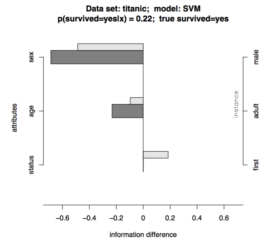
Robnik-Sikonja and Kononenko (2008) proposed to explain the model prediction for one instance by measuring the difference between the original prediction and the one made with omitting a set of features.

Let’s say we need to generate an explanation for a classification model f:X→Y. Given a data point x∈X which consists of a individual values of attribute Ai, i=1,…,a, and is labeled with class y∈Y. The prediction difference is quantified by computing the difference between the model predicted probabilities with or without knowing Ai:

probDiffi(y|x)=p(y|x)−p(y|x∖Ai)

(The paper also discussed on using the odds ratio or the entropy-based information metric to quantify the prediction difference.)

Problem: If the target model outputs a probability, then great, getting p(y|x) is straightforward. Otherwise, the model prediction has to run through an appropriate post-modeling calibration to translate the prediction score into probabilities. This calibration layer is another piece of complication.

Another problem: If we generate x∖Ai by replacing Ai with a missing value (like None, NaN, etc.), we have to rely on the model’s internal mechanism for missing value imputation. A model which replaces these missing cases with the median should have output very different from a model which imputes a special placeholder. One solution as presented in the paper is to replace Ai with all possible values of this feature and then sum up the prediction weighted by how likely each value shows in the data:p(y|x∖Ai)=∑s=1mip(Ai=as|x∖Ai)p(y|x←Ai=as)≈∑s=1mip(Ai=as)p(y|x←Ai=as)

Where p(y|x←Ai=as) is the probability of getting label y if we replace the feature Ai with value as in the feature vector of x. There are mi unique values of Ai in the training set.

With the help of the measures of prediction difference when omitting known features, we can decompose the impact of each individual feature on the prediction.

Local Gradient Explanation Vector

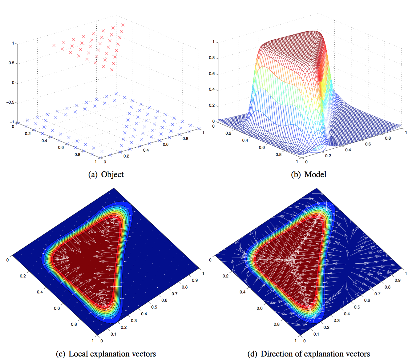
This method (Baehrens, et al. 2010) is able to explain the local decision taken by arbitrary nonlinear classification algorithms, using the local gradients that characterize how a data point has to be moved to change its predicted label.

Let’s say, we have a Bayes Classifier which is trained on the data set X and outputs probabilities over the class labels Y, p(Y=y|X=x). And one class label y is drawn from the class label pool, {1,2,…,C}. This Bayes classifier is constructed as:

f∗(x)=arg⁡minc∈{1,…,C}p(Y≠c|X=x)

The local explanation vector is defined as the derivative of the probability prediction function at the test point x=x0. A large entry in this vector highlights a feature with a big influence on the model decision; A positive sign indicates that increasing the feature would lower the probability of x0 assigned to f∗(x0).

However, this approach requires the model output to be a probability (similar to the “Prediction Decomposition” method above). What if the original model (labelled as f) is not calibrated to yield probabilities? As suggested by the paper, we can approximate f by another classifier in a form that resembles the Bayes classifier f∗:

(1) Apply Parzen window to the training data to estimate the weighted class densities:

p^σ(x,y=c)=1n∑i∈Ickσ(x−xi)

Where Ic is the index set containing the indices of data points assigned to class c by the model f, Ic={i|f(xi)=c}. kσ is a kernel function. Gaussian kernel is a popular one among many candidates.

(2) Then, apply the Bayes’ rule to approximate the probability p(Y=c|X=x) for all classes:p^σ(y=c|x)=p^σ(x,y=c)p^σ(x,y=c)+p^σ(x,y≠c)≈∑i∈Ickσ(x−xi)∑ikσ(x−xi)

(3) The final estimated Bayes classifier takes the form:

f^σ=arg⁡minc∈{1,…,C}p^σ(y≠c|x)

Noted that we can generate the labeled data with the original model f, as much as we want, not restricted by the size of the training data. The hyperparameter σ is selected to optimize the chances of f^σ(x)=f(x) to achieve high fidelity.

Side notes: As you can see both the methods above require the model prediction to be a probability. Calibration of the model output adds another layer of complication.

LIME (Local Interpretable Model-Agnostic Explanations)

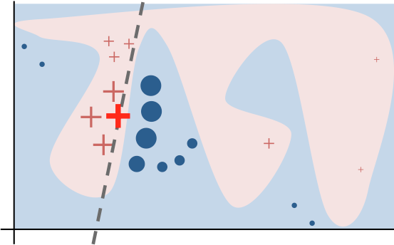
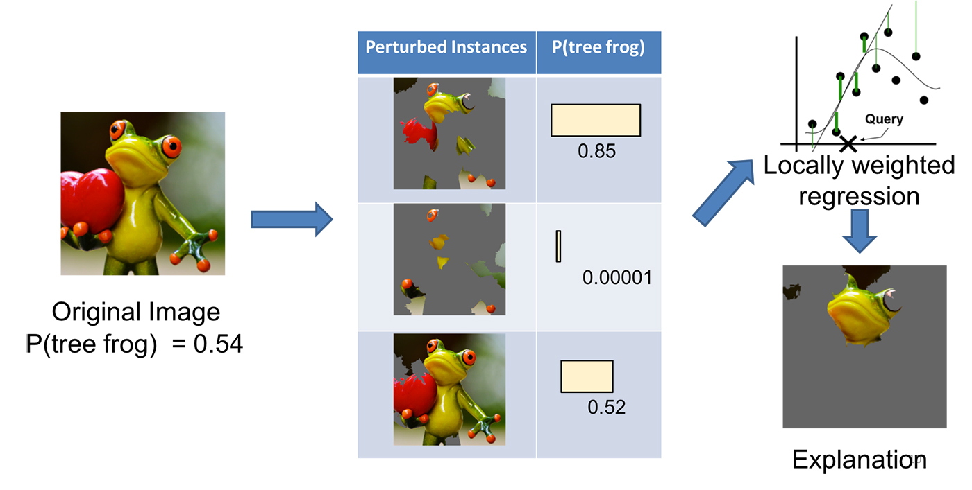
LIME, short for local interpretable model-agnostic explanation, can approximate a black-box model locally in the neighborhood of the prediction we are interested (Ribeiro, Singh, & Guestrin, 2016).

Same as above, let us label the black-box model as f. LIME presents the following steps:

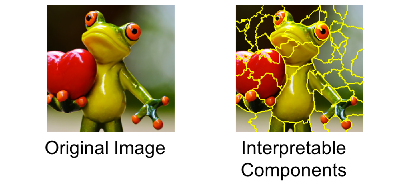
(1) Convert the dataset into interpretable data representation: x⇒xb.

• Text classifier: a binary vector indicating the presence or absence of a word
• Image classifier: a binary vector indicating the presence or absence of a contiguous patch of similar pixels (super-pixel).

(2) Given a prediction f(x) with the corresponding interpretable data representation xb, let us sample instances around xb by drawing nonzero elements of xb uniformly at random where the number of such draws is also uniformly sampled. This process generates a perturbed sample zb which contains a fraction of nonzero elements of xb.

Then we recover zb back into the original input z and get a prediction score f(z) by the target model.

Use many such sampled data points zb∈Zb and their model predictions, we can learn an explanation model (such as in a form as simple as a regression) with local fidelity. The sampled data points are weighted differently based on how close they are to xb. The paper used a lasso regression with preprocessing to select top k most significant features beforehand, named “K-LASSO”.

Examining whether the explanation makes sense can directly decide whether the model is trustworthy because sometimes the model can pick up spurious correlation or generalization. One interesting example in the paper is to apply LIME on an SVM text classifier for differentiating “Christianity” from “Atheism”. The model achieved a pretty good accuracy (94% on held-out testing set!), but the LIME explanation demonstrated that decisions were made by very arbitrary reasons, such as counting the words “re”, “posting” and “host” which have no connection with neither “Christianity” nor “Atheism” directly. After such a diagnosis, we learned that even the model gives us a nice accuracy, it cannot be trusted. It also shed lights on ways to improve the model, such as better preprocessing on the text.

For more detailed non-paper explanation, please read this blog post by the author. A very nice read.

Side Notes: Interpreting a model locally is supposed to be easier than interpreting the model globally, but harder to maintain (thinking about the curse of dimensionality). Methods described below aim to explain the behavior of a model as a whole. However, the global approach is unable to capture the fine-grained interpretation, such as a feature might be important in this region but not at all in another.

Feature Selection

Essentially all the classic feature selection methods (Yang and Pedersen, 1997; Guyon and Elisseeff, 2003) can be considered as ways to explain a model globally. Feature selection methods decompose the contribution of multiple features so that we can explain the overall model output by individual feature impact.

There are a ton of resources on feature selection so I would skip the topic in this post.

BETA (Black Box Explanation through Transparent Approximations)

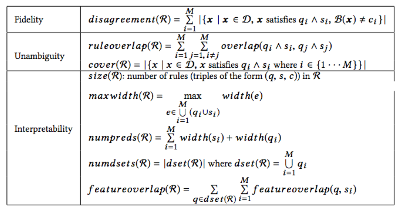
BETA, short for black box explanation through transparent approximations, is closely connected to Interpretable Decision Sets (Lakkaraju, Bach & Leskovec, 2016). BETA learns a compact two-level decision set in which each rule explains part of the model behavior unambiguously.

The authors proposed an novel objective function so that the learning process is optimized for high fidelity (high agreement between explanation and the model), low unambiguity (little overlaps between decision rules in the explanation), and high interpretability (the explanation decision set is lightweight and small). These aspects are combined into one objection function to optimize for.

Explainable Artificial Intelligence

I borrow the name of this section from the DARPA project “Explainable Artificial Intelligence”. This Explainable AI (XAI) program aims to develop more interpretable models and to enable human to understand, appropriately trust, and effectively manage the emerging generation of artificially intelligent techniques.

With the progress of the deep learning applications, people start worrying about that we may never know even if the model goes bad. The complicated structure, the large number of learnable parameters, the nonlinear mathematical operations and some intriguing properties (Szegedy et al., 2014) lead to the un-interpretability of deep neural networks, creating a true black-box. Although the power of deep learning is originated from this complexity — more flexible to capture rich and intricate patterns in the real-world data.

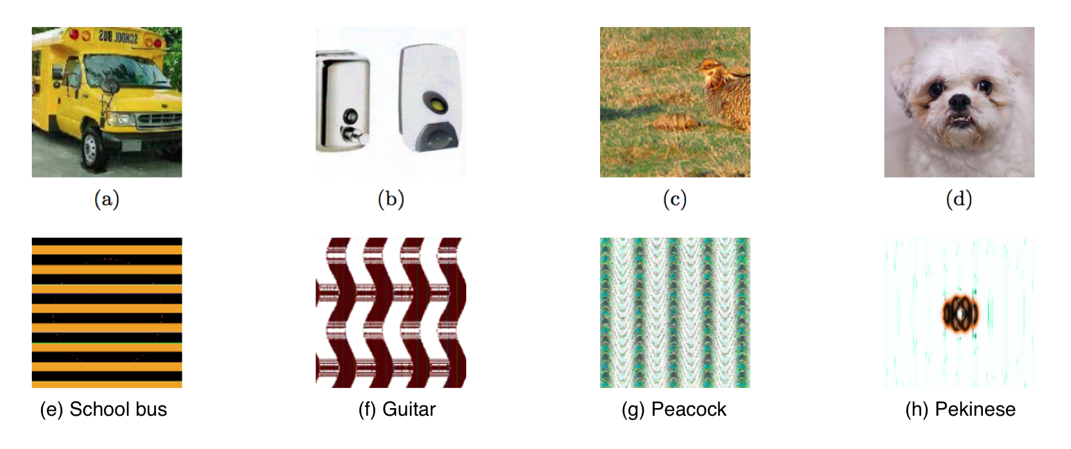
Studies on adversarial examples (OpenAI Blog: Robust Adversarial Examples, Attacking Machine Learning with Adversarial Examples, Goodfellow, Shlens & Szegedy, 2015; Nguyen, Yosinski, & Clune, 2015) raise the alarm on the robustness and safety of AI applications. Sometimes the models could show unintended, unexpected and unpredictable behavior and we have no fast/good strategy to tell why.

Nvidia recently developed a method to visualize the most important pixel points in their self-driving cars’ decisioning process. The visualization provides insights on how AI thinks and what the system relies on while operating the car. If what the AI believes to be important agrees with how human make similar decisions, we can naturally gain more confidence in the black-box model.

Many exciting news and findings are happening in this evolving field every day. Hope my post can give you some pointers and encourage you to investigate more into this topic 🙂

---

Cited as:

@article{weng2017gan,
  title   = "How to Explain the Prediction of a Machine Learning Model?",
  author  = "Weng, Lilian",
  journal = "lilianweng.github.io",
  year    = "2017",
  url     = "https://lilianweng.github.io/posts/2017-08-01-interpretation/"
}

References

[1] Zachary C. Lipton. “The mythos of model interpretability.” arXiv preprint arXiv:1606.03490 (2016).

[2] Been Kim, Rajiv Khanna, and Oluwasanmi O. Koyejo. “Examples are not enough, learn to criticize! criticism for interpretability.” Advances in Neural Information Processing Systems. 2016.

[3] Himabindu Lakkaraju, Stephen H. Bach, and Jure Leskovec. “Interpretable decision sets: A joint framework for description and prediction.” Proc. 22nd ACM SIGKDD Intl. Conf. on Knowledge Discovery and Data Mining. ACM, 2016.

[4] Robnik-Šikonja, Marko, and Igor Kononenko. “Explaining classifications for individual instances.” IEEE Transactions on Knowledge and Data Engineering 20.5 (2008): 589-600.

[5] Baehrens, David, et al. “How to explain individual classification decisions.” Journal of Machine Learning Research 11.Jun (2010): 1803-1831.

[6] Marco Tulio Ribeiro, Sameer Singh, and Carlos Guestrin. “Why should I trust you?: Explaining the predictions of any classifier.” Proc. 22nd ACM SIGKDD Intl. Conf. on Knowledge Discovery and Data Mining. ACM, 2016.

[7] Yiming Yang, and Jan O. Pedersen. “A comparative study on feature selection in text categorization.” Intl. Conf. on Machine Learning. Vol. 97. 1997.

[8] Isabelle Guyon, and André Elisseeff. “An introduction to variable and feature selection.” Journal of Machine Learning Research 3.Mar (2003): 1157-1182.

[9] Ian J. Goodfellow, Jonathon Shlens, and Christian Szegedy. “Explaining and harnessing adversarial examples.” ICLR 2015.

[10] Christian Szegedy, Wojciech Zaremba, Ilya Sutskever, Joan Bruna, Dumitru Erhan, Ian Goodfellow, Rob Fergus. “Intriguing properties of neural networks.” Intl. Conf. on Learning Representations (2014)

[11] Nguyen, Anh, Jason Yosinski, and Jeff Clune. “Deep neural networks are easily fooled: High confidence predictions for unrecognizable images.” Proc. IEEE Conference on Computer Vision and Pattern Recognition. 2015.

[12] Benjamin Letham, Cynthia Rudin, Tyler H. McCormick, and David Madigan. “Interpretable classifiers using rules and Bayesian analysis: Building a better stroke prediction model.” The Annals of Applied Statistics 9, No. 3 (2015): 1350-1371.

[13] Haohan Wang, Bhiksha Raj, and Eric P. Xing. “On the Origin of Deep Learning.” arXiv preprint arXiv:1702.07800 (2017).

[14] OpenAI Blog: Robust Adversarial Examples

[15] Attacking Machine Learning with Adversarial Examples

[16] Reading an AI Car’s Mind: How NVIDIA’s Neural Net Makes Decisions